Optimisation for machine learning

Why a whole lesson on optimisation#

Training a model = solving \(\min_\theta J(\theta)\). Lesson 02 did it for a quadratic bowl. Real costs are curved valleys (neural networks), or come with constraints (SVMs in lesson 05, probabilities that must sum to one, physical limits). This lesson collects the tools; later lessons just use them.

A hard test function#

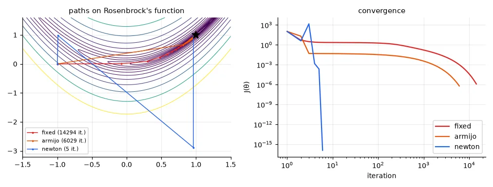
Rosenbrock's "banana" function has its minimum \(J=0\) at \((1,1)\), at the bottom of a long, narrow, curved valley — the kind of geometry that makes simple methods struggle:

def J(t):
    """Rosenbrock's banana function: minimum J = 0 at (1, 1), at the bottom of a curved valley."""
    return (1 - t[0]) ** 2 + 100 * (t[1] - t[0] ** 2) ** 2


def grad(t):
    return np.array([-2 * (1 - t[0]) - 400 * t[0] * (t[1] - t[0] ** 2),
                     200 * (t[1] - t[0] ** 2)])


def hessian(t):
    return np.array([[2 - 400 * t[1] + 1200 * t[0] ** 2, -400 * t[0]],
                     [-400 * t[0], 200]])

Hand-written derivatives are a classic source of silent bugs (a wrong sign still "trains", just badly). Always compare them once against finite differences, \(\partial J/\partial\theta_i \approx \big(J(\theta + h e_i) - J(\theta - h e_i)\big)/2h\):

def numerical_grad(f, t, h=1e-6):
    """Central finite differences: slow, but a reliable check of a hand-written gradient."""
    e = np.eye(len(t))
    return np.array([(f(t + h * e[i]) - f(t - h * e[i])) / (2 * h) for i in range(len(t))])


t = np.array([-0.7, 0.4])
print("analytic gradient", grad(t), "| numerical", numerical_grad(J, t).round(6))
print("analytic Hessian row 0", hessian(t)[0], "| numerical",
      numerical_grad(lambda s: grad(s)[0], t).round(4))

analytic gradient [-28.6 -18. ] | numerical [-28.6 -18. ]
analytic Hessian row 0 [430. 280.] | numerical [430. 280.]

Deep learning frameworks compute gradients automatically (lesson 12), and torch.autograd.gradcheck does exactly this test.

Three ways down the valley#

All descent methods iterate \(\theta_{k+1} = \theta_k + \alpha_k\, \mathbf{d}_k\); they differ in the direction \(\mathbf{d}_k\) and the step \(\alpha_k\).

• Gradient descent, fixed step. \(\mathbf{d} = -\nabla J\), \(\alpha\) constant. The step must be small enough for the steepest part of the valley, so it is far too small everywhere else.
• Gradient descent + Armijo backtracking. Start with \(\alpha = 1\) and halve it until the cost decreases "enough": \(J(\theta + \alpha\mathbf{d}) \le J(\theta) + c\,\alpha\,\nabla J^\top \mathbf{d}\). The step adapts to the local landscape at the price of a few extra evaluations of \(J\).
• Newton's method. Approximate \(J\) by its second-order Taylor expansion and jump to the minimum of that quadratic: \(\mathbf{d} = -H^{-1}\nabla J\), \(\alpha = 1\). The Hessian \(H\) rescales each direction by its curvature — the cure for the elongated valleys of lesson 02.

def armijo(theta, d, g, alpha=1.0, rho=0.5, c=1e-4):
    """Backtracking: halve the step until J decreases at least c * alpha * (slope along d)."""
    while J(theta + alpha * d) > J(theta) + c * alpha * g @ d:
        alpha *= rho
    return alpha


def minimise(theta0, method, tol=1e-3, max_iter=20000):
    theta = theta0.astype(float).copy()
    path = [theta.copy()]
    for it in range(max_iter):
        g = grad(theta)
        if np.linalg.norm(g) <= tol:
            break
        if method == "fixed":
            theta = theta - 1e-3 * g                         # fixed step size
        elif method == "armijo":
            theta = theta + armijo(theta, -g, g) * -g        # steepest descent + line search
        elif method == "newton":
            theta = theta - np.linalg.solve(hessian(theta), g)  # jump to the minimum of the local quadratic
        path.append(theta.copy())
    return theta, np.array(path), it


theta0 = np.array([-1.0, 0.0])
results = {}
for method in ("fixed", "armijo", "newton"):
    theta, path, it = minimise(theta0, method)
    results[method] = path
    print(f"{method:6s}: {it:5d} iterations -> theta = {np.round(theta, 4)}, J = {J(theta):.2e}")

fixed : 14294 iterations -> theta = [0.9989 0.9978], J = 1.25e-06
armijo:  6029 iterations -> theta = [0.9992 0.9984], J = 6.22e-07
newton:     5 iterations -> theta = [1. 1.], J = 2.07e-17

If Newton is so fast, why does nobody train neural networks with it? Because \(H\) has \(p^2\) entries for \(p\) parameters: for a network with 10⁷ weights that is 10¹⁴ numbers, and solving with it costs \(O(p^3)\). Deep learning uses first-order methods (SGD, Adam — lesson 12) that approximate the curvature cheaply, e.g. by normalising each parameter's step by the running size of its gradients.

Constraints: the Lagrangian and the dual#

Now minimise under inequality constraints:

The Lagrangian adds each constraint with a multiplier \(\mu_i \ge 0\): \(\mathcal{L}(\theta, \mu) = f(\theta) + \sum_i \mu_i g_i(\theta)\). At the optimum of a convex problem the KKT conditions hold: the gradient of \(\mathcal{L}\) is zero, constraints are satisfied, and complementary slackness \(\mu_i\, g_i(\theta^\star) = 0\) — a multiplier is non-zero only for constraints that are active (tight). Minimising \(\mathcal{L}\) over \(\theta\) first gives the dual problem in \(\mu\) alone. For convex problems both have the same optimal value (zero duality gap), so we can solve whichever is easier.

Example: projecting a point onto a polytope#

Find the point of the diamond \(|t_1| + |t_2| \le 1\) closest to \(c = (3, 1)\). Four linear constraints \(A\mathbf{t} \le \mathbf{b}\). CVXPY lets you write the problem as you would on paper and picks a solver:

# Project c onto the diamond |t1| + |t2| <= 1:  min 1/2 ||t - c||^2  s.t.  A t <= b
c = np.array([3.0, 1.0])
A = np.array([[1, 1], [1, -1], [-1, 1], [-1, -1]], dtype=float)
b = np.ones(4)

t = cp.Variable(2)
primal = cp.Problem(cp.Minimize(0.5 * cp.sum_squares(t - c)), [A @ t <= b])
primal.solve()
print("primal: t* =", np.round(t.value, 4), "objective", round(primal.value, 4))

Setting \(\nabla_t \mathcal{L} = (\mathbf{t} - \mathbf{c}) + A^\top\mu = 0\) gives \(\mathbf{t} = \mathbf{c} - A^\top \mu\); substituting back yields a quadratic problem in \(\mu \ge 0\):

# Lagrangian L(t, mu) = 1/2||t - c||^2 + mu^T (A t - b), mu >= 0.
# dL/dt = 0  ->  t = c - A^T mu.  Plugging it back gives the dual problem in mu only:
mu = cp.Variable(4)
dual = cp.Problem(cp.Minimize(0.5 * cp.quad_form(mu, A @ A.T) - (A @ c - b) @ mu), [mu >= 0])
dual.solve()
t_from_dual = c - A.T @ mu.value
print("dual: mu* =", np.round(mu.value, 4), "-> t = c - A^T mu =", np.round(t_from_dual, 4))
print("duality gap:", round(primal.value + dual.value, 6),
      "| multipliers from the primal solver:", np.round(primal.constraints[0].dual_value, 4))

primal: t* = [ 1. -0.] objective 2.5
dual: mu* = [1.5 0.5 0.  0. ] -> t = c - A^T mu = [1. 0.]
duality gap: 0.0 | multipliers from the primal solver: [1.5 0.5 0.  0. ]

Only the two constraints that meet at the vertex \((1, 0)\) have non-zero multipliers — complementary slackness in action. And CVXPY's primal solver hands us the same multipliers for free (constraint.dual_value). The dual is not a curiosity: in lesson 05 it is what turns a linear SVM into a kernel SVM.

The minimum enclosing ball#

Where do we put a fire station so that the farthest of 18 houses is as close as possible? Find the smallest ball (centre \(\mathbf{z}\), radius \(R\)) containing all points: \(\min R^2\) s.t. \(\|\mathbf{x}_i - \mathbf{z}\|^2 \le R^2\). Its dual is

The centre is a weighted average of the support points — the few points on the boundary, the only ones with \(\mu_i > 0\).

houses = np.loadtxt(U.path("houses.csv"), delimiter=",")     # (18, 2) coordinates


def enclosing_ball(X):
    """Minimum enclosing ball through its dual: max sum mu_i ||x_i||^2 - ||X^T mu||^2, mu in the simplex."""
    mu = cp.Variable(len(X))
    q = (X ** 2).sum(1)
    prob = cp.Problem(cp.Minimize(cp.sum_squares(X.T @ mu) - q @ mu), [mu >= 0, cp.sum(mu) == 1])
    prob.solve()
    mu = mu.value
    z = X.T @ mu                                   # centre = weighted mean of the support points
    support = mu > 1e-4
    r = np.sqrt(((X[support] - z) ** 2).sum(1).max())
    return z, r, support


z, r, sup = enclosing_ball(houses)
print("houses: centre %s, radius %.4f, %d support points" % (np.round(z, 4), r, sup.sum()))
outliers = np.array([[3.0, -3.0], [2.5, 2.5]])
z2, r2, sup2 = enclosing_ball(np.vstack([houses, outliers]))
print("with 2 outliers: centre %s, radius %.4f, %d support points" % (np.round(z2, 4), r2, sup2.sum()))

houses: centre [0. 0.], radius 1.4142, 4 support points
with 2 outliers: centre [ 1.65 -0.35], radius 2.9741, 3 support points

Two outliers move the centre and double the radius: the hard ball must contain everything. The fix is the same idea as the soft-margin SVM: allow points outside, but make them pay. With slack variables \(\xi_i \ge 0\),

def soft_ball(X, C):
    """Allow points outside the ball at a price: min R^2 + C sum(xi), ||x_i - z||^2 <= R^2 + xi."""
    z, R2, xi = cp.Variable(2), cp.Variable(), cp.Variable(len(X))
    cons = [cp.sum_squares(X[i] - z) <= R2 + xi[i] for i in range(len(X))] + [xi >= 0]
    cp.Problem(cp.Minimize(R2 + C * cp.sum(xi)), cons).solve()
    return z.value, np.sqrt(R2.value), xi.value > 1e-6


Xall = np.vstack([houses, outliers])
z3, r3, out3 = soft_ball(Xall, C=0.3)
print("soft ball (C = 0.3): centre %s, radius %.4f, points left outside: %s"
      % (np.round(z3, 4), r3, np.flatnonzero(out3)))

soft ball (C = 0.3): centre [ 1.2499 -0.    ], radius 2.4621, points left outside: [18 19]

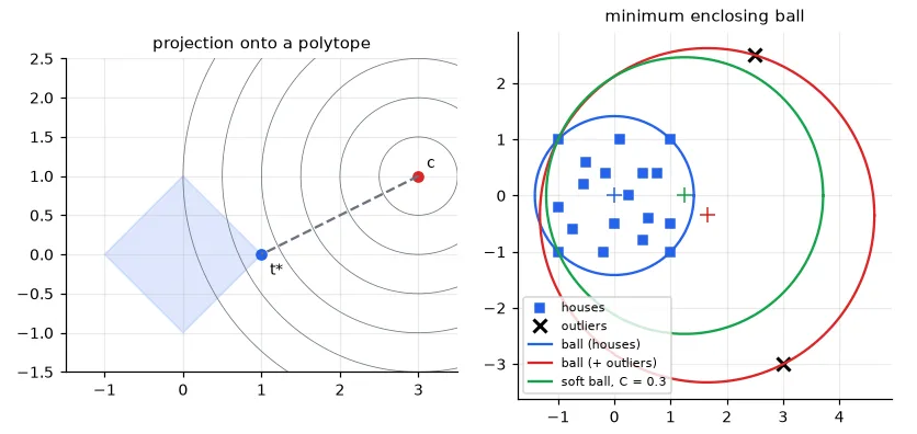
The soft ball leaves the outliers out, but it is still bigger and off-centre: an outlier outside the ball keeps pulling on the centre, with a force proportional to \(C\). Lower \(C\) and the ball shrinks further — but starts excluding houses too. \(C\) is a hyper-parameter: it sets the price of an error, and only validation data can tell you the right price. This model — a soft ball around "normal" data — is the Support Vector Data Description, used for anomaly detection.

Exercises#

1. Implement momentum: \(\mathbf{v} \leftarrow \beta \mathbf{v} - \alpha\nabla J\), \(\theta \leftarrow \theta + \mathbf{v}\) with \(\beta = 0.9\). How many iterations on Rosenbrock with a fixed \(\alpha\)?
2. Newton fails when \(H\) is not positive definite (try \(\theta_0 = (0, 1)\) and print the eigenvalues of \(H\)). Add damping: solve \((H + \lambda I)\mathbf{d} = -\nabla J\) with \(\lambda\) large enough.
3. Make the soft ball robust in two steps: fit it, drop the points with \(\xi_i > 0\), refit the hard ball on what is left. Do you recover the houses-only ball?