06 · Edge detection · Computer Vision Course

Edges in one dimension#

Take one row of an image. An edge is a jump in intensity. Its derivative — for discrete signals, the difference between neighbours, np.diff — is:

a peak at the edge, for the first derivative;
a positive/negative pair that crosses zero at the edge, for the second derivative.

step = np.r_[np.zeros(50), np.full(50, 255)]                  # sharp edge
ramp = np.r_[np.zeros(48), [25, 75, 175, 225], np.full(48, 250)]  # smooth edge
line = np.r_[np.zeros(47), [25, 75, 175, 250, 175, 75, 25], np.zeros(46)]  # thin line

d1 = np.diff(ramp)         # first derivative: a peak on the edge
d2 = np.diff(ramp, n=2)    # second derivative: + then -, crossing zero on the edge

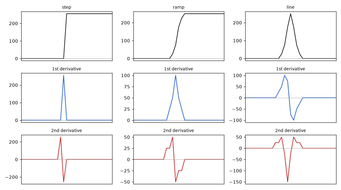
A sharp step, a smooth ramp and a thin line, with their first and second derivatives. Note that a thin *line* gives two first-derivative peaks of opposite sign.

So there are two families of edge detectors: look for maxima of the first derivative, or for zero crossings of the second.

The gradient#

In 2-D, the first derivative becomes the gradient, a vector of two partial derivatives:

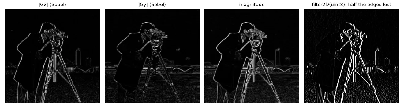
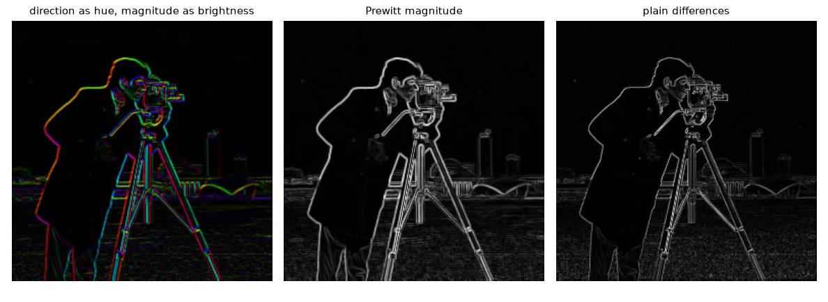
\[\nabla I = \left(\frac{\partial I}{\partial x}, \frac{\partial I}{\partial y}\right), \qquad |\nabla I| = \sqrt{G_x^2 + G_y^2}, \qquad \theta = \operatorname{atan2}(G_y, G_x)\]

The magnitude says how strong the edge is, the direction is perpendicular to the edge. Plain differences $I(x+1) - I(x)$ are very sensitive to noise, so practical operators combine a derivative in one direction with a smoothing in the other. Prewitt smooths with $[1, 1, 1]$, Sobel with $[1, 2, 1]$:

\[S_x = \begin{bmatrix} -1 & 0 & 1 \\ -2 & 0 & 2 \\ -1 & 0 & 1 \end{bmatrix}, \qquad S_y = S_x^\top\]

f = img.astype(np.float32)          # derivatives are signed: never compute them in uint8

dx = np.zeros_like(f)
dy = np.zeros_like(f)
dx[:, :-1] = np.diff(f, axis=1)     # I(x+1, y) - I(x, y)
dy[:-1, :] = np.diff(f, axis=0)     # I(x, y+1) - I(x, y)

sobel_x = np.array([[-1, 0, 1], [-2, 0, 2], [-1, 0, 1]], np.float32)
prewitt_x = np.array([[-1, 0, 1], [-1, 0, 1], [-1, 0, 1]], np.float32)

gx = cv2.filter2D(f, cv2.CV_32F, sobel_x)      # ddepth=CV_32F keeps negative values
gy = cv2.filter2D(f, cv2.CV_32F, sobel_x.T)
magnitude = np.hypot(gx, gy)                   # sqrt(gx² + gy²); |gx| + |gy| is a cheaper variant
direction = np.arctan2(gy, gx)                 # radians, perpendicular to the edge

# OpenCV shortcut, same numbers:
gx_cv = cv2.Sobel(f, cv2.CV_32F, 1, 0, ksize=3)

The classic bug

cv2.filter2D(img, -1, kernel) on a uint8 image returns uint8: every negative response is clipped to 0. Half of the edges (those going from bright to dark) disappear. Always ask for a float output (cv2.CV_32F, or cv2.CV_64F with cv2.Sobel).

$|G_x|$ responds to vertical edges, $|G_y|$ to horizontal ones, the magnitude to both. The last panel is the clipped `uint8` version: only one side of each edge survives.

Left: gradient direction as colour, magnitude as brightness — the two sides of the coat have opposite colours (opposite directions). Prewitt is visually almost identical to Sobel; plain differences are noisier.

Second derivatives: the Laplacian#

The Laplacian sums the two second derivatives, $\nabla^2 I = \partial^2 I/\partial x^2 + \partial^2 I/\partial y^2$, and is approximated by

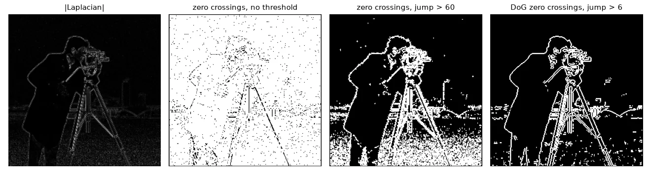
\[L_4 = \begin{bmatrix} 0 & -1 & 0 \\ -1 & 4 & -1 \\ 0 & -1 & 0 \end{bmatrix} \quad\text{or}\quad L_8 = \begin{bmatrix} -1 & -1 & -1 \\ -1 & 8 & -1 \\ -1 & -1 & -1 \end{bmatrix}\]

(sign conventions vary; only the zero crossings matter). It is isotropic — one kernel, no direction — but differentiating twice amplifies noise twice. The fix is to smooth first: the Laplacian of Gaussian (LoG), well approximated by the Difference of Gaussians (DoG), the same band-pass filter SIFT uses to find blobs in lesson 12.

lap4 = np.array([[0, -1, 0], [-1, 4, -1], [0, -1, 0]], np.float32)
lap8 = np.array([[-1, -1, -1], [-1, 8, -1], [-1, -1, -1]], np.float32)
laplacian = cv2.filter2D(f, cv2.CV_32F, lap4)


def gaussian_kernel(size, sigma):
    ax = np.arange(size) - size // 2
    xx, yy = np.meshgrid(ax, ax)
    k = np.exp(-(xx ** 2 + yy ** 2) / (2 * sigma ** 2))
    return k / k.sum()


# Difference of Gaussians: a band-pass filter that approximates the Laplacian of Gaussian
dog = (cv2.filter2D(f, cv2.CV_32F, gaussian_kernel(9, 1.0))
       - cv2.filter2D(f, cv2.CV_32F, gaussian_kernel(9, 1.6)))

Finding zero crossings#

A pixel is on an edge if one of its 4 neighbours has the opposite sign and the jump between them is large enough — without that second condition, every tiny ripple of noise around zero becomes an "edge".

def zero_crossings(resp, min_jump):
    """Edge where the sign changes between 4-neighbours AND the jump is large enough."""
    edges = np.zeros(resp.shape, bool)
    c = resp[1:-1, 1:-1]
    for n in (resp[:-2, 1:-1], resp[2:, 1:-1], resp[1:-1, :-2], resp[1:-1, 2:]):
        edges[1:-1, 1:-1] |= (np.sign(c) != np.sign(n)) & (np.abs(c - n) > min_jump)
    return edges

Without a threshold on the jump, the zero crossings of the Laplacian are everywhere. With it, the outlines appear, closed and one pixel thin. The DoG (smoothed first) gives cleaner contours.

First-order edges: threshold the magnitude#

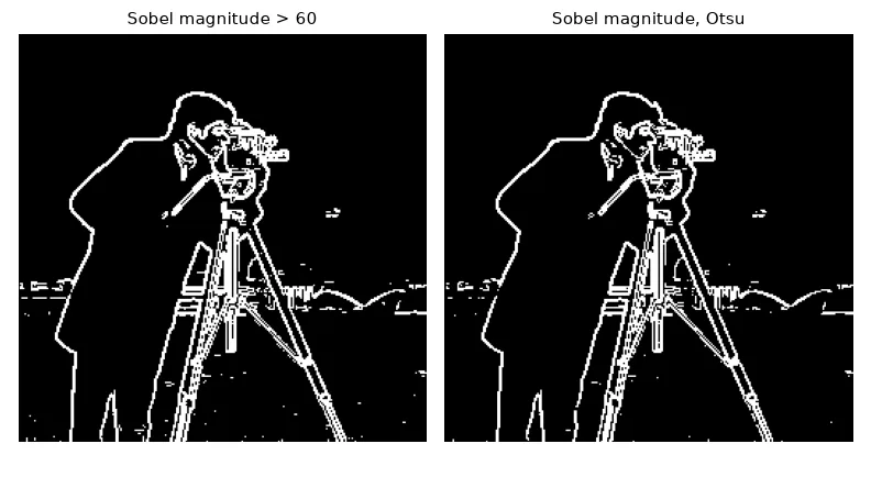
For first-order operators, edges are bright ridges of the magnitude, so a threshold is enough; Otsu's method picks it automatically by splitting the histogram into two classes with minimal variance.

def threshold(x, t):
    return (x >= t).astype(np.uint8) * 255


mag_u8 = to_u8(magnitude)
edges_sobel = threshold(mag_u8, 60)
_, edges_otsu = cv2.threshold(mag_u8, 0, 255, cv2.THRESH_BINARY + cv2.THRESH_OTSU)

Thresholded Sobel magnitude. The edges are thick (several pixels across) — lesson 07 thins them to exactly one pixel.

	First order (Sobel, Prewitt)	Second order (Laplacian, DoG)
Edge =	maximum of $	\nabla I
Gives	magnitude and direction	position only, no direction
Edges are	thick, need thinning	thin and closed
Noise	sensitive	very sensitive (smooth first)

A complete pipeline: noisy CT scan#

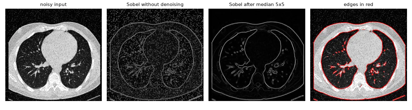
A real processing chain has three parts: pre-processing (fix the image), processing (extract the information), display. The CT slice below has salt-and-pepper noise, so lesson 05 tells us to start with a median filter:

brain = U.imread("noise/noisy_brain.png", cv2.IMREAD_GRAYSCALE)
den = cv2.medianBlur(brain, 5)                                   # 1. pre-processing: S&P noise
gx = cv2.Sobel(den, cv2.CV_32F, 1, 0)                            # 2. processing: gradient
gy = cv2.Sobel(den, cv2.CV_32F, 0, 1)
mag = to_u8(np.hypot(gx, gy))
_, edges = cv2.threshold(mag, 0, 255, cv2.THRESH_BINARY + cv2.THRESH_OTSU)
overlay = cv2.cvtColor(brain, cv2.COLOR_GRAY2BGR)                # 3. display: edges in red
overlay[edges > 0] = (0, 0, 255)

Without denoising, every impulse becomes a small ring of edges. After a 5×5 median, the Sobel magnitude shows the lungs, the heart and the vessels, and the thresholded edges are drawn in red on the input.

Exercises#

Compare $|G_x| + |G_y|$ and $\sqrt{G_x^2 + G_y^2}$: where do they differ most? (Hint: diagonal edges.)
Replace the DoG with cv2.Laplacian(cv2.GaussianBlur(f, (0, 0), 1.5), cv2.CV_32F) and tune the zero-crossing jump.
Draw the edges of noisy_brain.png in a different colour depending on the gradient direction (4 bins).