11 · Corners and tracking · Computer Vision Course

Why corners?#

To track motion, match two photos or calibrate a camera we need points that can be found again. A pixel in a flat region looks like all its neighbours; a pixel on an edge can slide along the edge without changing; only at a corner does any small move change the local appearance.

Make that precise: shift a window by $(u, v)$ and measure the change

\[E(u, v) = \sum_{x, y} w(x, y)\, [I(x + u, y + v) - I(x, y)]^2\]

A first-order Taylor expansion, $I(x+u, y+v) \approx I + I_x u + I_y v$, turns it into a quadratic form:

\[E(u, v) \approx \begin{bmatrix} u & v \end{bmatrix} M \begin{bmatrix} u \\ v \end{bmatrix}, \qquad M = \sum_{x, y} w(x, y) \begin{bmatrix} I_x^2 & I_x I_y \\ I_x I_y & I_y^2 \end{bmatrix} = \begin{bmatrix} S_{xx} & S_{xy} \\ S_{xy} & S_{yy} \end{bmatrix}\]

$M$ is the structure tensor. Its two eigenvalues $\lambda_1, \lambda_2$ say how much $E$ grows in the two principal directions: both small → flat; one large → edge; both large → corner.

Harris and Shi-Tomasi#

Computing eigenvalues at every pixel used to be expensive, so Harris and Stephens (1988) used a score built from the determinant and the trace, which are cheap:

\[R = \det M - k\,(\operatorname{tr} M)^2 = \lambda_1 \lambda_2 - k\,(\lambda_1 + \lambda_2)^2, \qquad k \approx 0.04\text{–}0.06\]

$R$ is large and positive at corners, negative on edges, near zero on flat areas. Shi and Tomasi (1994) used the smallest eigenvalue directly, $\min(\lambda_1, \lambda_2) = \tfrac{1}{2}\big(\operatorname{tr} M - \sqrt{(\operatorname{tr} M)^2 - 4 \det M}\big)$, which tracks better.

def structure_tensor(img, block=5, sigma=1.0):
    """Sxx, Sxy, Syy: Gaussian-weighted sums of gradient products around each pixel."""
    f = cv2.GaussianBlur(img.astype(np.float32), (3, 3), 0)      # tame the noise first
    ix = cv2.Sobel(f, cv2.CV_32F, 1, 0, ksize=3)
    iy = cv2.Sobel(f, cv2.CV_32F, 0, 1, ksize=3)
    sxx = cv2.GaussianBlur(ix * ix, (block, block), sigma)
    sxy = cv2.GaussianBlur(ix * iy, (block, block), sigma)
    syy = cv2.GaussianBlur(iy * iy, (block, block), sigma)
    return sxx, sxy, syy


def harris_response(img, k=0.05, block=5):
    sxx, sxy, syy = structure_tensor(img, block)
    det = sxx * syy - sxy ** 2          # lambda1 * lambda2
    trace = sxx + syy                   # lambda1 + lambda2
    return det - k * trace ** 2


def shi_tomasi_response(img, block=5):
    sxx, sxy, syy = structure_tensor(img, block)
    det = sxx * syy - sxy ** 2
    trace = sxx + syy
    return (trace - np.sqrt(np.maximum(trace ** 2 - 4 * det, 0))) / 2   # min(lambda1, lambda2)

The window $w$ is a Gaussian, so the sums become Gaussian blurs of the gradient products.

Non-maximum suppression#

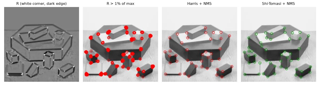
Thresholding $R$ gives blobs of candidates around each corner. Greedy NMS keeps the strongest candidate, forbids a square around it, and moves on:

def greedy_nms(response, rel_threshold=0.01, min_distance=10, max_corners=None):
    """Best candidate first; every accepted corner forbids a square around it."""
    ys, xs = np.nonzero(response > rel_threshold * response.max())
    order = np.argsort(response[ys, xs])[::-1]               # strongest first
    allowed = np.ones(response.shape, bool)
    corners = []
    for y, x in zip(ys[order], xs[order]):
        if allowed[y, x]:
            corners.append((x, y))
            allowed[max(0, y - min_distance):y + min_distance + 1,
                    max(0, x - min_distance):x + min_distance + 1] = False
            if max_corners and len(corners) == max_corners:
                break
    return np.array(corners, np.float32)

Harris: 554 pixels above threshold -> 41 corners after NMS

$R$ (white = corner, dark = edge); the 554 candidates; 41 corners after NMS; Shi-Tomasi with the same NMS.

The OpenCV way, and sub-pixel accuracy#

R_cv = cv2.cornerHarris(img.astype(np.float32), blockSize=5, ksize=3, k=0.05)   # the map only
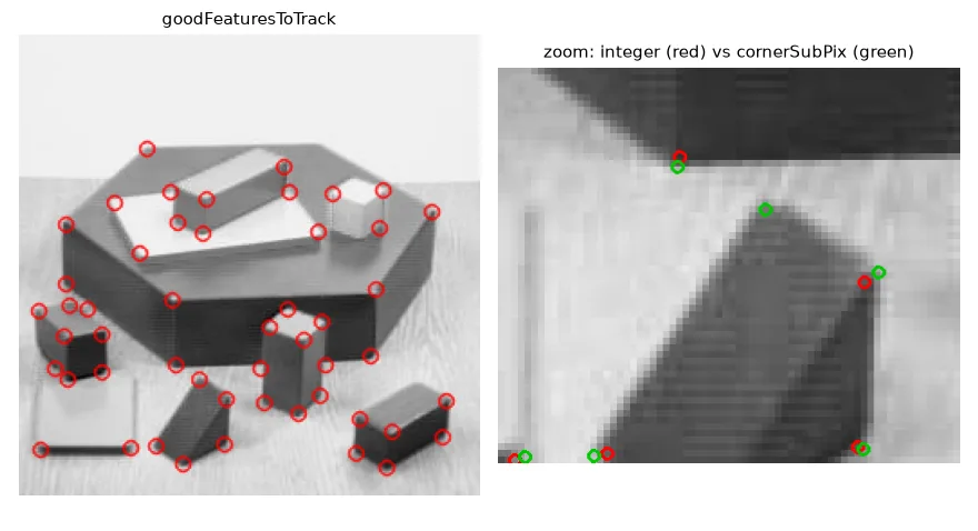
pts = cv2.goodFeaturesToTrack(img, maxCorners=50, qualityLevel=0.05, minDistance=8,
                              blockSize=5, useHarrisDetector=False)          # Shi-Tomasi + NMS
criteria = (cv2.TERM_CRITERIA_EPS + cv2.TERM_CRITERIA_MAX_ITER, 50, 0.001)
refined = cv2.cornerSubPix(img, pts.copy(), winSize=(5, 5), zeroZone=(-1, -1), criteria=criteria)

goodFeaturesToTrack is Shi-Tomasi (or Harris) + NMS + "keep the N best". Corners found on the pixel grid are only accurate to ±0.5 px, and the blur moves them further; cornerSubPix refines each one by finding the point where the image gradients around it are orthogonal to the vector towards it. Here corners moved by 1.9 px on average — huge for calibration (lesson 14), where we need ~0.1 px.

Integer corners (red) and refined ones (green) on a zoom of the blocks.

Tracking by template matching#

To follow a corner into the next frame, take a small patch around it and look for the most similar patch nearby. The similarity that does not care about brightness or contrast changes is the zero-mean normalised cross-correlation:

\[\mathrm{NCC}(T, W) = \frac{\sum (T - \bar T)(W - \bar W)}{\sqrt{\sum (T - \bar T)^2 \, \sum (W - \bar W)^2}} \in [-1, 1]\]

def ncc(a, b):
    """Zero-mean normalized cross-correlation of two equal-size patches, in [-1, 1]."""
    a = a.astype(np.float32) - a.mean()
    b = b.astype(np.float32) - b.mean()
    denom = np.sqrt((a * a).sum() * (b * b).sum())
    return float((a * b).sum() / denom) if denom > 0 else 0.0


def track_ncc(img0, img1, points, half=7, search=20):
    """For each point, find the patch of img1 (within +-search px) most similar to its patch in img0."""
    out = []
    for x, y in points.astype(int):
        tpl = img0[y - half:y + half + 1, x - half:x + half + 1]
        best, best_xy = -1.0, (x, y)
        for dy in range(-search, search + 1):
            for dx in range(-search, search + 1):
                yy, xx = y + dy, x + dx
                win = img1[yy - half:yy + half + 1, xx - half:xx + half + 1]
                if win.shape != tpl.shape:
                    continue
                score = ncc(tpl, win)
                if score > best:
                    best, best_xy = score, (xx, yy)
        out.append((*best_xy, best))
    return np.array(out, np.float32)

cv2.matchTemplate computes the NCC at every position of the search window at once:

x, y = p0[0].astype(int)
tpl = frame0[y - 7:y + 8, x - 7:x + 8]
area = frame1[y - 27:y + 28, x - 27:x + 28]                       # +-20 px search window
scores = cv2.matchTemplate(area, tpl, cv2.TM_CCOEFF_NORMED)       # same NCC, vectorised
_, best_score, _, best_loc = cv2.minMaxLoc(scores)

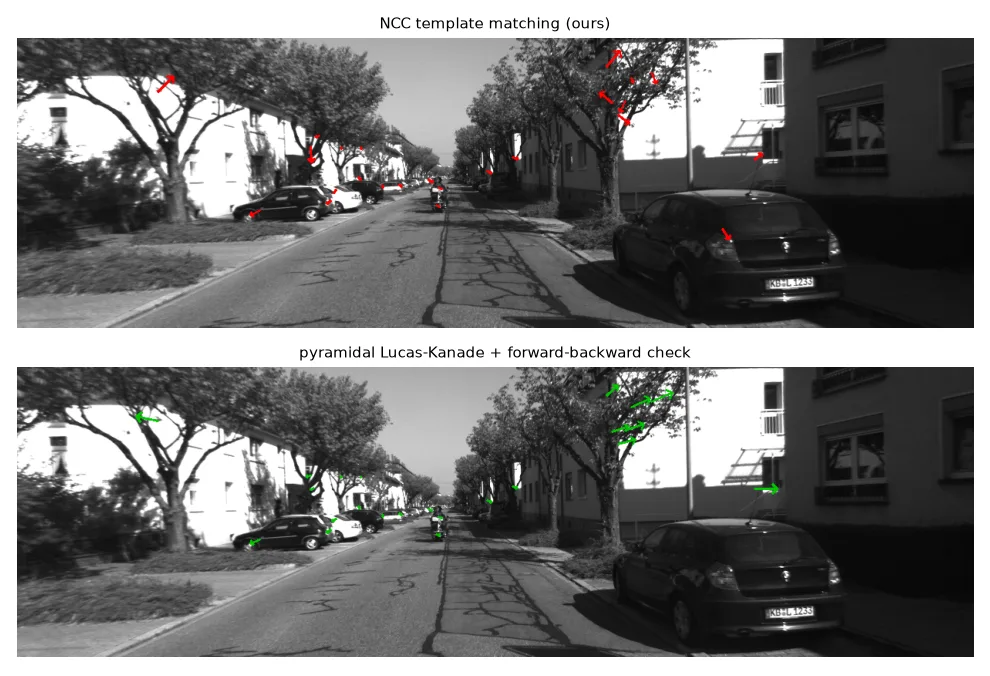
Both find the same position with the same score (0.849).

Lucas-Kanade optical flow#

Template search costs $O(\text{window}^2)$ per point. Lucas-Kanade instead assumes brightness constancy, $I_x u + I_y v + I_t = 0$, writes one such equation per pixel of a small window and solves the least-squares system $M\,[u, v]^\top = -[\sum I_x I_t, \sum I_y I_t]^\top$ — the same structure tensor $M$. That is why it needs corners: on an edge $M$ is singular (the aperture problem). An image pyramid handles large motions by solving coarse-to-fine.

p0_lk = p0.reshape(-1, 1, 2)
p1_lk, status, err = cv2.calcOpticalFlowPyrLK(frame0, frame1, p0_lk, None,
                                              winSize=(21, 21), maxLevel=3)
# forward-backward check: track back to frame 0 and demand that we land where we started
p0_back, status_back, _ = cv2.calcOpticalFlowPyrLK(frame1, frame0, p1_lk, None,
                                                   winSize=(21, 21), maxLevel=3)
fb_error = np.linalg.norm(p0_back - p0_lk, axis=2).ravel()
good = (status.ravel() == 1) & (status_back.ravel() == 1) & (fb_error < 1.0)

The forward-backward check tracks every point back to the first frame and rejects those that do not return home (here 2 of 25). It is the cheapest outlier filter there is.

KITTI frames 0 → 2. Points move away from the centre of the image as the car drives forward. NCC and Lucas-Kanade agree to 0.6 px (median) on the points LK kept.

Exercises#

Plot $\lambda_1$ vs $\lambda_2$ (computed with np.linalg.eigvalsh on $M$) for every pixel of blox.jpg and colour the points by Harris' $R$.
Track 200 corners through all 15 KITTI frames with LK, re-detecting new corners when fewer than 100 remain, and draw the tracks.
Make track_ncc vectorised with cv2.matchTemplate and compare speed.